Greedy algorithms

An optimization problem is one in which you want to find, not just a solution, but the best solution
A “greedy algorithm” sometimes works well for optimization problems
A greedy algorithm works in phases: At each phase:
- You take the best you can get right now, without regard for future consequences
- You hope that by choosing a local optimum at each step, you will end up at a global optimum

Example: Counting money

Suppose you want to count out a certain amount of money, using the fewest possible bills and coins
A greedy algorithm would do this would be:

At each step, take the largest possible bill or coin that does not overshoot

Example: To make $6.39, you can choose:

a $5 bill
a $1 bill, to make $6
a 25¢ coin, to make $6.25
a 10¢ coin, to make $6.35
four 1¢ coins, to make $6.39
For US money, the greedy algorithm always gives the optimum solution

However, greedy algorithms don't always work.

Consider in some (fictional) monetary system, “krons” come in 1 kron, 7 kron, and 10 kron coins
Using a greedy algorithm to count out 15 krons, you would get

A 10 kron piece
Five 1 kron pieces, for a total of 15 krons
This requires six coins
A better solution would be to use two 7 kron pieces and one 1 kron piece
This only requires three coins
The greedy algorithm results in a solution, but not an optimal solution

Spaning Trees

Suppose you own a telecom company and you're looking to lay cable in a new neighborhood. ...

A spanning tree T of a connected graph $G = (V,E)$ is a
subgraph of $G$ that is:

connected
acyclic
includes all of V as vertices.

The minimum spanning tree (MST) problem:
Suppose that we have a connected, undirected graph $G=(V,E)$ , with a numerical weighting $w(u,v)$ for each edge $(u,v)$ .
Problem: Find an acyclic subset $T \subseteq E$ that connects all of the vertices in $V$ , and minimizes:
$\Sigma \{w(u,v) | (u,v) \in T\}$

Solution: We will look for an algorithm of the form:
$E_T \leftarrow$ empty set of edges
while ( $E_T$ is not a spanning tree)
- add an edge to $E_T$
At each stage we will ensure that $E_T$ is a subset of a MST

Test yourself

If $e$ is a minimum-weight edge in a connected
graph, then $e$ must be an edge in at least one
minimum spanning tree

True or False?

Must $e$ be an edge in all minimum
spanning trees of the graph?

If every edge in a connected graph $G$ has a
distinct weight, then $G$ must have a unique
minimum spanning tree?

Proof
Assume the contrary, that there are two different MSTs $A$ and $B$ .

Since $A$ and $B$ differ despite containing the same nodes, there is at least one edge that belongs to one but not the other. Among such edges, let $e1$ be the one with least weight; this choice is unique because the edge weights are all distinct. Without loss of generality, assume $e1$ is in $A$ .
As $B$ is an MST, $e1 \cup B$ must contain a cycle $C$ with $e1$ .
As a tree, $A$ contains no cycles, therefore $C$ must have an edge $e2$ that is not in $A$ .
Since $e1$ was chosen as the unique lowest-weight edge among those belonging to exactly one of $A$ and $B$ , the weight of $e2$ must be greater than the weight of $e1$ .
As $e1$ and $e2$ are part of the cycle $C$ , replacing $e2$ with $e1$ in $B$ therefore yields a spanning tree with a smaller weight.
This contradicts the assumption that $B$ is a MST.

Prim's Algorithm

Prim's

Idea: Construct a MST by greedily expanding an initial tree, composed of just a single vertex of the graph's vertices. To expand the tree, attach the nearest vertex, i.e. add the vertex connected by the lowest weight edge amongst the neighbors of the current expanding tree such that we don't create a cycle.

Pseudocode:
Input: A weighted connected graph $G = (V,E)$
Output: $E_r$ the set of edges composing a minimum spanning tree of G.

Prim(G):
$V_r \leftarrow {v_0}$
$E_r \leftarrow \varnothing$
for $i \leftarrow 1$ to $|V|- 1$ do:
    find a minimum-weight edge $e^* = (v^*, u^*)$ among all the edges $(v, u)$ such that $v$ is in $V_r$ and $u$ is in $V - V_r$
     $V_r \leftarrow V_r \cup \{u^*\}$
     $E_r \leftarrow E_r \cup \{e^*\}$
return $E_r$

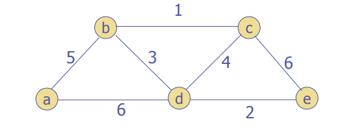
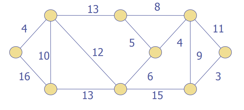
Let's try two examples

A bit more detail:

 1 The input is the graph G=(V, E), and a root r in V.
 2 for each v in V
 3   key[v] ← ∞;
 4   parent[v] ← null;
 5 key[r] ← 0;
 6 add all vertices in V to the queue Q.
 7 while (Q is nonempty):
 8   u ← extractMin(Q);
 9   for each vertex v that is adjacent to u:
10     if v ∈ Q and weight(u,v) < key[v]:
11       parent[v] ← u;
12       key[v] ← weight(u,v);

Ideas: Store all vertices that are not in ( $V_T, E_T$ ) in a priority queue Q with an extractMin operation.
If u is a vertex in Q, what’s key[u] (the value that determines u’s position in Q)?
- key[u] = minimum weight of edge from u into $V_T$
- If no such edge exists, key[u] = ∞.
- We maintain information about the parent (in ( $V_T, E_T$ )) of each vertex v in an array parent[].
- $E_T$ is kept implicitly as {(v, parent[v]) | v ∈ V−Q−{r}}.

Complexity:
The operations that contribute most toward Prim's algorithm revolve around our data structure operations. The input size is measured by $|V|$ and $|E|$ .

Assuming a binary heap:

Initialization takes $\mathcal{O}(|V|)$ time.
Main loop is executed $|V|$ times, and each extractMin takes $\mathcal{O}(\log |V|)$ .
The body of the inner loop is executed a total of $\mathcal{O}(|E|)$ times; each adjustment of the queue takes \mathcal{O}(\log |V|)$ time.
Overall complexity: $\mathcal{O}((|V|+|E|) \log |V|) = \mathcal{O}(|E| \log |V|)$ .

Kruskal's Algorithm

Kruskal's

Idea: create a forest F (a set of trees), where each vertex in the graph is a separate tree
create a set S containing all edges in the graph
while S is not empty ad F is not yet spanning:
-remove and edge with minimum weight from S
-if the removed edge connects to different trees, then add it to F, combining two trees into a single tree
At the termination of the algorithm, the forest forms a minimum spanning tree of the graph.

Pseudocode using the union find data structure:

Kruskal(G):
1  A = null
2  for each v in V:
3    MakeSet(v)
4  for each (u, v) in E, sorted by weight from smallest to largest:
5    if FindSet(u) != FindSet(v):
6      A = A union {(u, v)}
7      Union(u, v)
8  return A

Union Find (disjoint set) data structure
The operations we need are:

Make a singleton set;

Test if two sets are equal;

Union two sets together.

Complexity:
The operations that contribute most toward the run time of Kruskal's are:
(1) sorting the edges and (2) the union find operations.

Sorting the edges costs $\mathcal{O}(|E| \log |E|)$ time.

The union find data structure can perform $\mathcal{O}(|V|)$ operations in $\mathcal{O}(|V| \log |V|)$ time.

A sophisticated union find data structure can run in $\mathcal{O}(\alpha (|V|))$ time.
Combined with a linear time sorting algorithm, we could achieve $\mathcal{O}(|E| \alpha(|V|))$ run time.

Shortest path - Dijkstra’s Algorithm

Dijkstra's

Dijkstra’s finds the lowest cost path from source node and a destination node in a weighted graph. More generally, it finds the shortest path from a source node to every node.

Idea: First, it finds the shortest path from the source to a vertex nearest to it, then to a second nearest, and so on. In general, before its $i^{th}$ iteration commences, the algorithm has already identified the shortest paths to $i − 1$ other vertices nearest to the source.

Begin by setting the distance of every node from the source node to infinity and the source node to 0. Then consider the closest unvisited node. (On the first iteration, this will be the source node.) From this node, update the distance to every unvisited neighbor. The update is done by comparing the distance of the node plus the edge to the neighbor to the distance of the neighbor. Update the value if smaller, mark the current node as the parent in the shortest path, and mark the current node as being visited. Repeat until all nodes are visited.

Input: A source node s and destination node d, Graph G =
(V, E) with edge weights {length(u, v) for (u, v) in E}
Output: the path weight from s to d

 1  function Dijkstra(Graph, source):
 2
 3      create vertex set Q
 4
 5      for each vertex v in Graph:             
 6          dist[v] ← INFINITY                  
 7          prev[v] ← UNDEFINED                 
 8          add v to Q                      
10      dist[source] ← 0                        
11      
12      while Q is not empty:
13          u ← vertex in Q with min dist[u]    
14                                              
15          remove u from Q
16          
17          for each neighbor v of u:           
18              alt ← dist[u] + length(u, v)
19              if alt < dist[v]:               
20                  dist[v] ← alt
21                  prev[v] ← u
22
23      return dist[], prev[]

Using a min priority queue, we can get better efficiency. Instead of searching for the min vertex in $Q$ , $Q$ could be implemented as a min priority queue and we'd extract the min from $Q$ and update it - with a decrease-key operation - at each step.

Complexity: (See Dijsktra's on Wikipedia)
Like Prim's and Kruskal's this algorithm's run time primarily depends upon the operations on the data structures. The input size is measured by the number of vertices and edges in the graph.

For any implementation of the vertex set $Q$ , the running time is in:

$\mathcal{O}(|E|\cdot T_{dk}+|V|\cdot T_{em})$

where $T_{dk}$ and $T_{em}$ are the complexities of the decrease-key and extract-minimum operations in $Q$ , respectively. The simplest implementation of Dijkstra's algorithm stores the vertex set $Q$ as an ordinary linked list or array, and extract-minimum is simply a linear search through all vertices in $Q$ . In this case, the running time is $\mathcal{O}(|E|+|V|^{2})= \mathcal{O}(|V|^{2})$ .

With a self-balancing binary search tree or binary heap, the algorithm improves to:

$\Theta ((|E|+|V|)\log |V|)$

For connected graphs, this can be simplified to $\Theta(|E| \log |V|)$

In an implementation of Dijkstra's algorithm that supports decrease-key, the priority queue holding the nodes begins with $|V| = n$ nodes in it and on each step of the algorithm removes one node. This means that the total number of heap dequeues is $n$ . Each node will have decrease-key called on it potentially once for each edge leading into it, so the total number of decrease-keys done is at most $m$ . This gives a runtime of $(n T_e + n T_d + m T_k)$ , where $T_k$ is the time required to call decrease-key.

Queue	$T_e$	$T_d$	$T_k$	w/o Dec-Key	w/Dec-Key
Array/LL	$n$			$\mathcal{O}(n^2)$
Binary Heap	$\mathcal{O}(\log n)$	$\mathcal{O}(\log n)$	$\mathcal{O}(\log n)$	$\mathcal{O}(m \log n)$	$\mathcal{O}(m \log n)$
Fibonacci Heap	$\mathcal{O}(1)$	$\mathcal{O}(\log n)$	$\mathcal{O}(1)$	$\mathcal{O}(m \log n)$	$\mathcal{O}(m + n \log n)$