Quicksort

Quicksort is an efficient sorting algorithm, developed by British computer scientist Tony Hoare.

Like Merge sort it is also a divide and conquer method. However, while merge sort divides the problem according to the position of the elements of the array, quicksort divides them according to the element's value.

Basic idea:

1. Pick an element from the array, called the pivot.
2. Partition: reorder the array so that all elements with values less than the pivot come before the pivot, while all elements with values greater than the pivot come after it (equal values can go either way). After this partitioning, the pivot is in its final position.
3. Recurse on the lower subarray and the upper subarray.

Quicksort(A[l...r]):
  if l < r:
    s <- Partition(A[l...r])
    Quicksort(A[l...s-1])
    Quicksort(A[s+1...r])

Lomuto Partition

This scheme is attributed to Nico Lomuto and popularized in Cormen et al. in their book Introduction to Algorithms (CLRS).

This scheme chooses a pivot that is typically the last element in the array. The algorithm maintains index i as it scans the array using another index j such that the elements lo through i (inclusive) are less than or equal to the pivot, and the elements i+1 through j-1 (inclusive) are greater than the pivot.

This scheme degrades to O(n2) when the array is already in order.

LomutoPartition(A[l...r]):
  p<-A[l]
  s<-l
  for i <- l+1 to r:
    if A[i] < p:
      s <- s+1
      swap(A[s], A[i])
  swap(A[l], A[s])
  return s

Hoare Partition

The original partition scheme described by Tony Hoare uses two indices that start at the ends of the array being partitioned, then move toward each other, until they detect an inversion: a pair of elements, one greater than or equal to the pivot, one lesser or equal, that are in the wrong order relative to each other. The inverted elements are then swapped. When the indices meet, the algorithm stops and returns the final index.

HoarePartition(A[l...r]):
  p <- A[l]
  i <- l
  j <- r+1
  do until i >= j:
    do until A[i] >= p:
      i <- i+1
    do until A[j] <= p:
      j < j-1
    swap(A[i], A[j])
  swap(A[i], A[j])
  swap(A[l], A[j])
  return j

Input size: length of array
Basic operation: comparisons

Best case not same as worst case:
If all partitions happen in the middle of corresponding subarrays, we get the best case.

$C_{best}(n) = 2C_{best}(n/2) + n$ for $n > 1$, $C_{best}(1) = 0$

Using the Master Theorem, $a = 2$, $b = 2$, and $c = 1$, we get case 2:

$C_{best}(n) \in \Theta(n^d \log n) = \Theta(n \log n)$

In the worst case, all partitions are skewed with one subarray being empty and the other 1 less than the size of the subarray being partitioned. This can occur if the pivot happens to be the smallest or largest element in the list or if all the elements are the same (as in the case of Lomuto Partition). If this happens repeatedly in every partition, then each recursive call processes a list of size one less than the previous list. So we make $n-1$ nested calls before we reach a list of size 1. So the call tree is a linear chain of $n-1$ nested calls.

The $i$th call does $\Theta(n - i)$ work for the partition, so:

$\sum_{i=0}^n (n-i) = \sum_{i=0}^n n - \sum_{i=0}^n i = n^2 - \frac{n(n-1)}{2} = \frac{n(n+1)}{2} \in \Theta(n^2)$

In the average case, the number of comparisons made by quicksort on a randomly ordered array is such that a partition can happen in any position $s$ where $0 \leq s \leq n-1$ after $n+1$ comparisons are made to achieve the partition. After the partition, the left and right subarrays will have $s$ and $n - 1 - s$ elements, respectively. Assuming that the partition split can happen in each position $s$ with the same probability $\frac{1}{n}$, we get the following recurrence relation:

$C_{avg}(n) = \frac{1}{n}\sum_{s=0}^{n-1}[(n+1) + C_{avg}(s) + C+{avg}(n-1-s)]$ for $n>1$
$C_{avg}(0) = 0$ and $C_{avg}(1) = 0$

This turns out to be: $C_{avg}(n) \approx 2n \ln n \approx 1.39n \log_2 n$

So on average, quicksort makes only 39% more comparisons than in the best case.

Refinements:

• Better pivot selection:
  • Randomized quicksort
  • median-of-three
  • median of medians (median of 5)
• Switching to insertion sort on very small subarrays (between 5 and 15 elements) or not sorting small subarrays at all and finishing with insertion sort applied to a nearly sorted array.
• Modifying the partition algorithm
  • three way partition

Weakness:

• not stable

Heap Sort

Priority Queue: An abstract data type, like a queue or stack, but where each element also has a priority associated with it. In a priority queue, an element with high priority is served before an element with low priority. In some implementations, elements with equal priority are served according to the order which they were enqueued. A naïve implementation, using an unsorted list provides $\mathcal{O}(1)$ insertion time and $\mathcal{O}(n)$ retrieval time. Priority queues are often implemented by a heap, which improves performance to $\mathcal{O}(n \log n)$ insertion and retrieval and $\mathcal{O}(n)$ initial build time.

Heaps themselves are often implemented as a complete binary tree, i.e. all of its levels are full except the last one which is filled left to right. The tree needs to preserve the heap property, on which each parent is greater than or equal to the children. So the root is always the largest element.

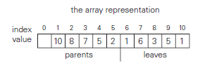
The tree is then laid out flat in an array. If we leave the first element empty:

• the parent node keys will be in the first floor($\frac{n}{2}$) positions of the array while the leaves will occupy the last ceil($\frac{n}{2}$) positions.
• the children of a key in the array's parental position $i$ ($1 \leq i \leq$ floor($\frac{n}{2})$) will be in positions $2i$ and $2i + 1$, and correspondingly, the parent of a key in position $i$ ($2 \leq i \leq n$) will be in position floor($\frac{i}{2}$)

For example:

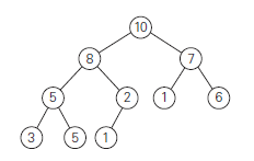
For the most part, we can just think of heaps as a binary tree with the right shape property and the heap property enforced.

Constructing a heap can be done in a number of ways, primarily top down or bottom up. The top down approach consists of building the heap while maintaining the heap property one item at a time. This has a $\mathcal{O}(n\log n)$ run time. The bottom up approach builds a compete tree with all of the items and then heapifys the tree to establish the heap property. This has a $\mathcal{O}(n)$ run time.

Heapsort is a two stage algorithm:

1. Constrct a heap for a given array.
2. Then sort by repeating until the heap has only one element left:

• Swap the first element (i.e. the root/the largest) with the last element.
• Heapify the heap portion of the array to maintain heap property

Heapsort Analysis:
Heap construction is $\mathcal{O}(n)$.
What is the second stage run time? We need to know the number of comparisons needed to heapify after removing the root element of the heap which diminishes in size from $n$ to $2$. The textbook gives us the following inequality:

$C(n) \leq 2$ floor($\log_2 (n-1)$) $+ 2$ floor($\log_2 (n - 2)$) $+ ... + 2$ floor($2 \log_2 1$) $\leq 2 \sum_{i=1}^{n-1} \log_2 i$
$\leq 2\sum_{i=1}^{n-1} \log_2 (n-1) = 2(n-1) \log_2(n-1) \leq 2n \log_2 n$ $\in \mathcal{O}(n \log n)$ for stage 2.

So for both stages we get:
$\mathcal{O}(n) + \mathcal{O}(n \log n) = \mathcal{O}(n \log n)$

In both worst and average cases, heapsort is $\Theta(n \log n)$

Count Sort

Count sort is a sorting technique based on keys between a specific range (small integers). The idea is to count the number of items having distinct key values, kind of like hashing, and then doing some arithmetic to calculate the position of each item in the output sequence.

DistributionCounting(A, l, u)
// Input: An array A[0..n − 1] of integers between l and u
//Output: Array S[0..n − 1] of A’s elements sorted in nondecreasing order
for j ← 0 to u − l:
  D[j] ← 0                      //initialize frequencies
for i ← 0 to n − 1:
  D[A[i] − l] ← D[A[i] − l] + 1 //compute frequencies
for j ← 1 to u − l:
  D[j] ← D[j − 1]+ D[j]         //reuse for distribution
for i ← n − 1 down to 0:
  j ← A[i]− l
  S[D[j]− 1] ← A[i]
  D[j] ← D[j]− 1
return S

The first loop initializes an array of $u-l$ 0s. The second loop goes over the items in the array, computing a histogram of the number of times each key occurs. The third loop computes a prefix sum of that count to determine, for each key, the positional range where the items having that key should be placed. Finally, the last loop moves each item into its sorted position in the output array S while decrementing the count for that key.

Analysis:
Pretty straightforward. Initialization of the count array D and the third loop, performing the prefix sum each iterate at most u-l + 1 times. Let $k = u - l$. So that's $\Theta(k)$ time. We make two consecutive passes through the input array, which each take $\Theta(n)$ time. So $2 \Theta(k) + 2 \Theta(n) = \Theta(n + k)$

Radix sort

Idea: sort data with integer keys by grouping keys by the individual digits which share the same significant position and value.

Least Significant Digit Radix Sort

1. Take the least significant digit of each key.
2. Group the keys based on that digit, keeping their order.
3. Collect the groups in the order of the digits and repeat the process wit the next least significant digit.

Example:
Ones place:
170, 45, 75, 90, 02, 802, 2, 66

170, 90, 02, 802, 2, 45, 75, 66

Tens place:
02, 802, 2, 45, 66, 170, 75, 90

Hundreds:
02, 2, 45, 66, 75, 90, 170, 802

Importantly, each of the above steps requires just a single pass over the data, since each item can be placed in its correct bucket without needing to compare to other items.

Analysis:

We need to make a pass over the entire list for each digit (or word size) of the key. Take $n$ to be the list size and $w$ to be the word size:
$\Theta(nw)$

In many cases, $w$ is very limited, so might as well be a constant.

Other interesting sorting Algorithms

Binary tree sort:

1. Construct a binary tree out of the items
2. Flatten the tree