Insertion Sort

Decrease and Conquer technique

• Decrease by a constant
  • Calculating factorial $f(n) = f(n-1) * n$
• Decrease by a constant factor
  • Binary search (decrease by half or factor of 2)
• Variable size decrease
  • Euclid's algorithm for computing gcd: $\gcd(m,n) = \gcd(n, m \mod n)$

Decrease by one -- Insertion Sort
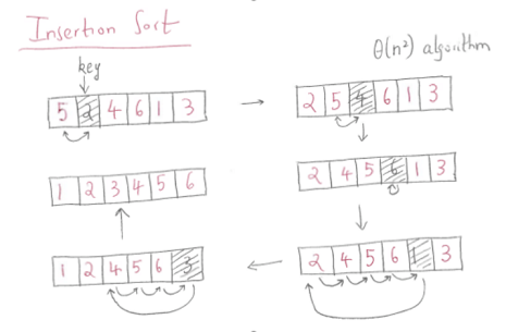
The idea is to divide the array into two subsets - sorted and unsorted. Initially the sorted subset consists of only one first element at index 0. Then for each iteration, insertion sort removes the next element from the unsorted subset, finds the location it belongs within the sorted subset, and inserts it there.

for i <- 1 ... n-1:
  v <- A[i]
  j <- i-1
  while j >= 0 and A[j] > v:
    A[j+1] <- A[j]
    j <- j - 1
  A[j+1] <- v

Example:

Basic Op: Comparison
In the worst case A[j] > v is executed for every j = i -1, ..., 0.
$C_{worst}(n) = \sum_{i=1}^{n-1} \sum_{j=0}^{i-1} 1 = \sum_{i=1}^{n-1}i = \frac{n(n-1)}{2} \in \Theta(n^2)$

In the best case, A[j] > v is executed only once on every iteration of the outer loop, i.e. if the input is already sorted.
$C_{best}(n) = \sum_{i=1}^{n-1} 1 = n-1 \in \Theta(n)$

Note that while we can't expect input to be sorted, almost insertion sort still works very efficiently on almost sorted inputs.

Average case: based on the probability of element pairs that are out of order.
$C_{avg} \approx \frac{n^2}{4} \in \Theta(n^2)$ (Twice as fast as worst case)

Improvements?
Instead of linearly scanning the sorted partition for the correct position to insert, binary search for the position.
However, the number of swaps in the worst case is still the same $\mathcal{O}(n^2)$

Merge Sort

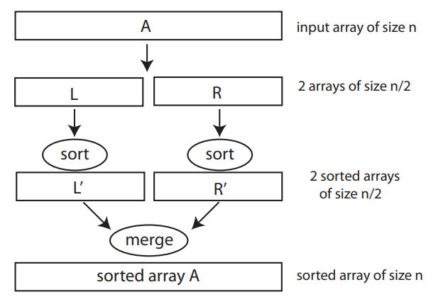
Divide and Conquer

Master Theorem

Let an instance of size $n$ be divided into $b$ instances of size $\frac{n}{b}$, with $a$ of them needing to be solved. (Let $a$ and $b$ be constants; $a \geq 1$ and $b \geq 1$). Assuming that size $n$ is a power of $b$ to simplify our analysis, we get the following recurrence relation for running time $T(n)$:
$T(n) = aT(\frac{n}{b}) + f(n)$

where $f(n)$ is a function that accounts for the time spend on dividing an instance of size $n$ into instances of size $\frac{n}{b}$ and combining their solutions.

If $f(n) \in \Theta(n^d)$ where $d \geq 0$ in recurrence, then

$t(n) \in \{$
$\Theta(n^d)$ if $a < b^d$
$\Theta(n^d \log n)$ if $a = b^d$
$\Theta(n^{\log_b a})$ if $a > b^d$
$\}$

Remember:

• $a$ is the nubmer of subproblems
• $\frac{n}{b}$ is the size of each subproblem
• $f(n)$ is the cost of dividing the problem into subproblems and merging the solutions of the subproblems.

Example:
Divide and Conquer Sum-Computation Algorithm
Divide list of numbers in two recursively sum them together.

$A(n) = 2A(\frac{n}{2}) + 1$
So $a = 2$, $b=2$ and $d=0$, so $a > b^d$
So $A(n) \in \Theta(n^{\log_2 2}) = \Theta(n ^{\log_2 2}) = \Theta(n)$

Another Example:
Binary Search

Recurrence relation for BS is:
$B(n) = B(\frac{n}{2}) + 1$
So $a = 1$, $b = 2$, and $d=0$, so $a = b^d$
So $B(n) \in \Theta(n^d \log n) = \Theta(\log n)$

---

Back to Merge Sort

mergesort(A):
  if n > 1:
    copy A[0...floor(n/2) - 1] to B[0...floor(n/2) - 1]
    copy A[floor(n/2)...n-1] to C[0...ceil(n/2) - 1]
    mergesort(B[0...floor(n/2)-1])
    mergesort(C[0... ceil(n/2)-1])
    merge(B, C, A)

Merging is done in the following way:
Two pointers are initialized to point to the first elements of the arrays being merged. The elements pointed to are compared and the smaller of them is added to the new array being constructed. After that the index of the smaller element is incremented to point to its successor in the array it was copied from. Repeat until one of the two is finished. The remaining from the other array can be copied to the end of the merged array.

merge(B[0...p-1], C[0...q-1], A[0...p+q-1]):
  while i < p and j < p:
    if B[i] <= C[j]:
      A[k] <- B[i]
      i <- i+1
    else:
      A[k] <- c[j]
      j <- j+1
    k <- k+1
  if i = p:
    copy C[j...q-1] to A[k...p+q-1]
  else:
    copy B[i...p-1] to A[k...p+q-1]

Analysis:
Basic operation: key comparisons
$C(n) = 2C(\frac{n}{2}) + C_{merge}(n)$ for $n > 1$, $C(1) = 0$

$T(n) = C_1 + 2T(\frac{n}{2}) + Cn$
where $C_1$ is the time it takes to divide
$2T(\frac{n}{2})$ is the running time for the recursive work
and $Cn$ is the time it takes to merge

$T(n) = 2T(\frac{n}{2}) + Cn + C_1$
$= 2(2T(\frac{n}{4}) + C\frac{n}{2} + C_1) + Cn + C_1 = 2^2 T(\frac{n}{2^2}) 2Cn + (1 + 2)C_1$
$= ... = 2^3T(\frac{n}{2^3}) + 3Cn + (1 + 2 + 2^2)C_1$
$= ...$
$= 2^k T(\frac{n}{2^k}) + kCn + (1 + 2 + 2^2 + ... + 2^{k-1})C_1$
$=$ (assuming $n = 2^k$) $nT(1) + \log_2 nCn + (n-1)C_1 = \Theta(n \log_2 n)$

Using master theorem:

$T(n) = aT(\frac{n}{b}) + f(n)$ where $a = 2$, $b = 2$, $d = 1$
$= \Theta(n \log n)$ since $a = b^d$ i.e., $2 = 2^1$

Solved in the book for more exact count of operations:
p173.
$C_{worst}(n) = n \log_2 n - n + 1$

Quicksort

Quicksort is an efficient sorting algorithm, developed by British computer scientist Tony Hoare.

Like Merge sort it is also a divide and conquer method. However, while merge sort divides the problem according to the position of the elements of the array, quicksort divides them according to the element's value.

Basic idea:

1. Pick an element from the array, called the pivot.
2. Partition: reorder the array so that all elements with values less than the pivot come before the pivot, while all elements with values greater than the pivot come after it (equal values can go either way). After this partitioning, the pivot is in its final position.
3. Recurse on the lower subarray and the upper subarray.

Quicksort(A[l...r]):
  if l < r:
    s <- Partition(A[l...r])
    Quicksort(A[l...s-1])
    Quicksort(A[s+1...r])

Lomuto Partition

This scheme is attributed to Nico Lomuto and popularized in Cormen et al. in their book Introduction to Algorithms (CLRS).

This scheme chooses a pivot that is typically the last element in the array. The algorithm maintains index i as it scans the array using another index j such that the elements lo through i (inclusive) are less than or equal to the pivot, and the elements i+1 through j-1 (inclusive) are greater than the pivot.

This scheme degrades to O(n2) when the array is already in order.

LomutoPartition(A[l...r]):
  p<-A[l]
  s<-l
  for i <- l+1 to r:
    if A[i] < p:
      s <- s+1
      swap(A[s], A[i])
  swap(A[l], A[s])
  return s

Hoare Partition

The original partition scheme described by Tony Hoare uses two indices that start at the ends of the array being partitioned, then move toward each other, until they detect an inversion: a pair of elements, one greater than or equal to the pivot, one lesser or equal, that are in the wrong order relative to each other. The inverted elements are then swapped. When the indices meet, the algorithm stops and returns the final index.

HoarePartition(A[l...r]):
  p <- A[l]
  i <- l
  j <- r+1
  do until i >= j:
    do until A[i] >= p:
      i <- i+1
    do until A[j] <= p:
      j < j-1
    swap(A[i], A[j])
  swap(A[i], A[j])
  swap(A[l], A[j])
  return j

Input size: length of array
Basic operation: comparisons

Best case not same as worst case:
If all partitions happen in the middle of corresponding subarrays, we get the best case.

$C_{best}(n) = 2C_{best}(n/2) + n$ for $n > 1$, $C_{best}(1) = 0$

Using the Master Theorem, $a = 2$, $b = 2$, and $c = 1$, we get case 2:

$C_{best}(n) \in \Theta(n^d \log n) = \Theta(n \log n)$

In the worst case, all partitions are skewed with one subarray being empty and the other 1 less than the size of the subarray being partitioned. This can occur if the pivot happens to be the smallest or largest element in the list or if all the elements are the same (as in the case of Lomuto Partition). If this happens repeatedly in every partition, then each recursive call processes a list of size one less than the previous list. So we make $n-1$ nested calls before we reach a list of size 1. So the call tree is a linear chain of $n-1$ nested calls.

The $i$th call does $\Theta(n - i)$ work for the partition, so:

$\sum_{i=0}^n (n-i) = \sum_{i=0}^n n - \sum_{i=0}^n i = n^2 - \frac{n(n-1)}{2} = \frac{n(n+1)}{2} \in \Theta(n^2)$

Heap Sort

Count Sort

* [Master Theorem](#master-theorem)