Sorting

Remember:
Before we can think about developing an algorithm, we have to agree on what problem our algorithm is supposed to solve.

We need to determine if our problem statement carries any hidden assumptions, and state those assumptions explicitly.

We may need to refine our specification as we develop the algorithm. For instance, our algorithm may require a particular input representations or produce particular output representations that were unspecified in the problem.

Sorting in Computer Science is the problem of arranging some items in a data structure in an ordered sequence

Sorting is a common operation in many applications.

• Efficient lookup and searching
• Efficient merging of sequences
• Enables processing of data in a defined order

Problem: Given a list of n sortable items, rearrange them in nondecreasing order.

Things to think about: does it matter how our list is implemented? Does it matter what sort of things we're trying to sort?

Stability

A sorting algorithm is called stable if two objects with equal keys appear in the same order in the sorted output as they appear in the input. Some sorting algorithms are stable by nature (insertion sort, merge sort, bubble sort) and some aren't (selection, quicksort, heap sort).

Why would it matter?
Suppose we have a list of first and last names and we want to sort by last, then first. We could first sort by first name, then use a stable sort by last name. The expected output at the end of these two operations will be sorted by last, then first name.

---

Brute Force

Brute force in computer science is a very general problem-solving technique that consists of systematically generating all possible candidates for the solution and checking each to see whether it satisfies the problem statement.

For example:
Traveling Salesman Problem

Input: a list of $n$ cities, A, and an $n\times n$ matrix with distances between cities, D
Output: a permutation of A with the shortest possible route.

TSP Pseudocode:

bestDistance <- infinity
bestRoute <- []

for each permutation of A, P:
  distance <- RouteLength(P)
  if distance < bestDistance:
    bestDistance <- distance
    bestRoute <- P
return bestRoute

Basic op: generate a permutation
Running time? $\Theta(n!)$

https://xkcd.com/399/

---

Selection Sort

Scan the list to find its smallest element and exchange it with the first element. Then scan the list, starting with the second element to find the smallest amongst the remaining n-1 elements and exchange it with the second element.

Generally: on the $i$th pass through the list, scan for the smallest item amongst the remaining $n-i$ elements and swap it with $A_i$

After $n-1$ passes, the list is sorted.

for i <- 0... n-2:
  min <- i
  for j <- i+1 ... n-1:
    if A[j] < A[min]:
      min <- j
    swap(A[i], A[min])

Examples

7 | 5 | 4 | 2
i = 0, min = 3
2 | 5 | 4 | 7
i = 1, min = 2
2 | 4 | 5 | 7
i = 2, min = 2

Is it stable? Yes
Selection Sort Analysis:
Input size: number of elements $n$
Basic operation: Key comparison
Best case/Worst case: Same

$C(n) = \sum_{i=0}^{n-2} \sum_{j=i+1}^{n-2} 1$
$= \sum_{i=0}^{n-2}[(n-1) - (i+1) +1] = \sum_{i=0}^{n-2}(n-1-i)$
$= \frac{n(n-1)}{2} \in \Theta(n^2)$

What about number of swaps?
$\mathcal{O}(n)$ swaps

---

Bubble Sort

Scan the list comparing adjacent elements of the list and exchange them if they are out of order. On the first pass, the largest element will be "bubbled up" to the end of the list. The next pass "bubbles up" the second largest element, and so on.

for i <- 0 ... n-2:
  for j <- 0 ... n-2-i:
    if A[j+1] < A[j]:
      Swap(A[j], A[j+1])

Insertion Sort

Decrease and Conquer technique

• Decrease by a constant
  • Calculating factorial $f(n) = f(n-1) * n$
• Decrease by a constant factor
  • Binary search (decrease by half or factor of 2)
• Variable size decrease
  • Euclid's algorithm for computing gcd: $\gcd(m,n) = \gcd(n, m \mod n)$

Decrease by one -- Insertion Sort
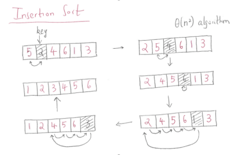
The idea is to divide the array into two subsets - sorted and unsorted. Initially the sorted subset consists of only one first element at index 0. Then for each iteration, insertion sort removes the next element from the unsorted subset, finds the location it belongs within the sorted subset, and inserts it there.

for i <- 1 ... n-1:
  v <- A[i]
  j <- i-1
  while j >= 0 and A[j] > v:
    A[j+1] <- A[j]
    j <- j - 1
  A[j+1] <- v

Example:

Basic Op: Comparison
In the worst case A[j] > v is executed for every j = i -1, ..., 0.
$C_{worst}(n) = \sum_{i=1}^{n-1} \sum_{j=0}^{i-1} 1 = \sum_{i=1}^{n-1}i = \frac{n(n-1)}{2} \in \Theta(n^2)$

In the best case, A[j] > v is executed only once on every iteration of the outer loop, i.e. if the input is already sorted.
$C_{best}(n) = \sum_{i=1}^{n-1} 1 = n-1 \in \Theta(n)$

Note that while we can't expect input to be sorted, almost insertion sort still works very efficiently on almost sorted inputs.

Average case: based on the probability of element pairs that are out of order.
$C_{avg} \approx \frac{n^2}{4} \in \Theta(n^2)$ (Twice as fast as worst case)

Improvements?
Instead of linearly scanning the sorted partition for the correct position to insert, binary search for the position.
However, the number of swaps in the worst case is still the same $\mathcal{O}(n^2)$

Merge Sort

Divide and Conquer

Master Theorem

Let an instance of size $n$ be divided into $b$ instances of size $\frac{n}{b}$, with $a$ of them needing to be solved. (Let $a$ and $b$ be constants; $a \geq 1$ and $b \geq 1$). Assuming that size $n$ is a power of $b$ to simplify our analysis, we get the following recurrence relation for running time $T(n)$:
$T(n) = aT(\frac{n}{b}) + f(n)$

where $f(n)$ is a function that accounts for the time spend on dividing an instance of size $n$ into instances of size $\frac{n}{b}$ and combining their solutions.

If $f(n) \in \Theta(n^d)$ where $d \geq 0$ in recurrence, then

$t(n) \in \{$
$\Theta(n^d)$ if $a < b^d$
$\Theta(n^d \log n)$ if $a = b^d$
$\Theta(n^{\log_b a})$ if $a > b^d$
$\}$

Remember:

• $a$ is the nubmer of subproblems
• $\frac{n}{b}$ is the size of each subproblem
• $f(n)$ is the cost of dividing the problem into subproblems and merging the solutions of the subproblems.

Example:
Divide and Conquer Sum-Computation Algorithm
Divide list of numbers in two recursively sum them together.

$A(n) = 2A(\frac{n}{2}) + 1$
So $a = 2$, $b=2$ and $d=0$, so $a > b^d$
So $A(n) \in \Theta(n^{\log_2 2}) = \Theta(n ^{\log_2 2}) = \Theta(n)$

Another Example:
Binary Search

Recurrence relation for BS is:
$B(n) = B(\frac{n}{2}) + 1$
So $a = 1$, $b = 2$, and $d=0$, so $a = b^d$
So $B(n) \in \Theta(n^d \log n) = \Theta(\log n)$

---

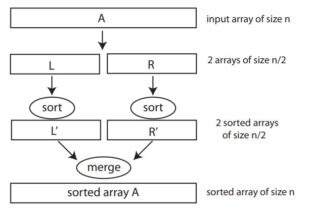
Back to Merge Sort

mergesort(A):
  if n > 1:
    copy A[0...floor(n/2) - 1] to B[0...floor(n/2) - 1]
    copy A[floor(n/2)...n-1] to C[0...ceil(n/2) - 1]
    mergesort(B[0...floor(n/2)-1])
    mergesort(C[0... ceil(n/2)-1])
    merge(B, C, A)

Merging is done in the following way:
Two pointers are initialized to point to the first elements of the arrays being merged. The elements pointed to are compared and the smaller of them is added to the new array being constructed. After that the index of the smaller element is incremented to point to its successor in the array it was copied from. Repeat until one of the two is finished. The remaining from the other array can be copied to the end of the merged array.

merge(B[0...p-1], C[0...q-1], A[0...p+q-1]):
  while i < p and j < p:
    if B[i] <= C[j]:
      A[k] <- B[i]
      i <- i+1
    else:
      A[k] <- c[j]
      j <- j+1
    k <- k+1
  if i = p:
    copy C[j...q-1] to A[k...p+q-1]
  else:
    copy B[i...p-1] to A[k...p+q-1]

Analysis:
Basic operation: key comparisons
$C(n) = 2C(\frac{n}{2}) + C_{merge}(n)$ for $n > 1$, $C(1) = 0$

$T(n) = C_1 + 2T(\frac{n}{2}) + Cn$
where $C_1$ is the time it takes to divide
$2T(\frac{n}{2})$ is the running time for the recursive work
and $Cn$ is the time it takes to merge

$T(n) = 2T(\frac{n}{2}) + Cn + C_1$
$= 2(2T(\frac{n}{4}) + C\frac{n}{2} + C_1) + Cn + C_1 = 2^2 T(\frac{n}{2^2}) 2Cn + (1 + 2)C_1$
$= ... = 2^3T(\frac{n}{2^3}) + 3Cn + (1 + 2 + 2^2)C_1$
$= ...$
$= 2^k T(\frac{n}{2^k}) + kCn + (1 + 2 + 2^2 + ... + 2^{k-1})C_1$
$=$ (assuming $n = 2^k$) $nT(1) + \log_2 nCn + (n-1)C_1 = \Theta(n \log_2 n)$

Using master theorem:

$T(n) = aT(\frac{n}{b}) + f(n)$ where $a = 2$, $b = 2$, $d = 1$
$= \Theta(n \log n)$ since $a = b^d$ i.e., $2 = 2^1$

Solved in the book for more exact count of operations:
p173.
$C_{worst}(n) = n \log_2 n - n + 1$

Quicksort

Heap Sort

Count Sort